Heuristic Search and Reinforcement Learning
Originally published in Chinese on 2020-12-10; this English edition preserves the original scope and technical context.
The Pac-Man Projects are a course project in UC Berkeley CS 188, where we will use this project to illustrate heuristic search and reinforcement learning.
1 Blind Search
Blind Search refers to search algorithms that do not utilize any additional information (input data or auxiliary functions) beyond the algorithm itself, such as BFS, DFS, Dijkstra, etc.
DFS
In search.py, we have already implemented the background logic and graphical rendering framework for Pac-Man. We need to implement the specific search algorithm and generate the path for Pac-Man to move. Let’s start by implementing a simple DFS:
python def dfs_search(start, goal, graph): path = [] stack = [(start, [start])] while stack: (node, path) = stack.pop() if node == goal: return path for neighbor in graph[node]: if neighbor not in path: stack.append((neighbor, path + [neighbor])) return None
def DepthFirstSearch(problem):
    from util import Stack
    open_list = Stack()
    visited = []
    open_list.push((problem.getStartState(), []))
    while not open_list.isEmpty():
        current_node, path = open_list.pop()
        if problem.isGoalState(current_node):
            return path
        if current_node in visited:
            continue
        visited.append(current_node)
        for next_node, action, cost in problem.getSuccessors(current_node):
            if next_node not in visited:
                open_list.push((next_node, path + [action]))
dfs = DepthFirstSearch
In the framework of the Pac-Man game, the problem parameter passed to the pathfinding function can be understood as an abstract base class class SearchProblem. The actual problems include PositionSearchProblem (finding a single goal), FoodSearchProblem (finding all food), and CapsuleSearchProblem (finding bonuses and all food). Each of these subclasses must implement the following functions:
getStartState(): Returns the initial state;isGoalState(state): Determines if thestatenode is a goal node;getSuccessors(state): Returns all successor nodes of thestatenode;getCostOfActions(actions): Given anactionslist consisting of up, down, left, and right directions, returns the total cost of the actions list.
Let’s run it to see the effect of DFS:
$ python pacman.py -l smallEmpty -z 0.8 -p SearchAgent -a fn=dfs
[SearchAgent] using function dfs
[SearchAgent] using problem type PositionSearchProblem
Path found with total cost of 56 in 0.002992 seconds
Search nodes expanded: 56
Pacman emerges victorious! Score: 454
Average Score: 454.0
Scores:        454.0
Win Rate:      1/1 (1.00)
Record:        Win
The parameter list running has several parameters:
-l smallEmpty:run on thesmallEmptymap, defined in thelayoutsdirectory;-z 0.8:client scaling factor is 0.8;-p SearchAgent:specify the actual problem, whereSearchAgentis a shorthand forfn='depthFirstSearch', prob='PositionSearchProblem'.
Actual running results are as follows:
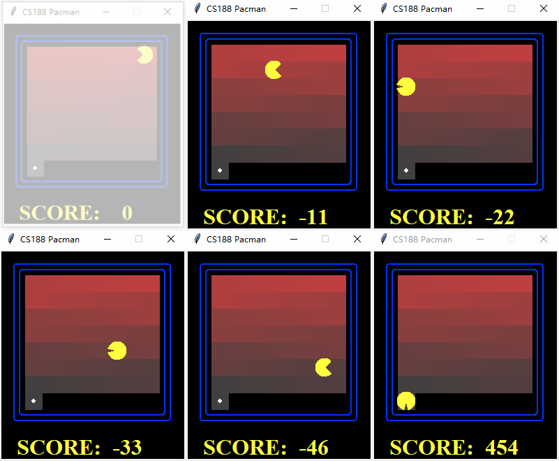
One can see that the Pac-Man agent took a long detour to reach the endpoint, as DFS is incomplete (and thus non-optimal) in computational complexity theory.
BFS
def BreadthFirstSearch(problem):
    from util import Queue
    open_list = Queue()
    visited = set()
    open_list.push((problem.getStartState(), []))
    while not open_list.isEmpty():
        current_node, path = open_list.pop()
        if problem.isGoalState(current_node):
            return path
        if current_node in visited:
            continue
        visited.add(current_node)
        for next_node, action, cost in problem.getSuccessors(current_node):
            if next_node not in visited:
                open_list.push((next_node, path + [action]))
bfs = BreadthFirstSearch
BFS performs as follows:
$ python pacman.py -l smallEmpty -z 0.8 -p SearchAgent -a fn=bfs
[SearchAgent] using function bfs
[SearchAgent] using problem type PositionSearchProblem
Path found with total cost of 14 in 0.001995 seconds
Search nodes expanded: 63
Pacman emerges victorious! Score: 496
Average Score: 496.0
Scores:        496.0
Win Rate:      1/1 (1.00)
Record:        Win
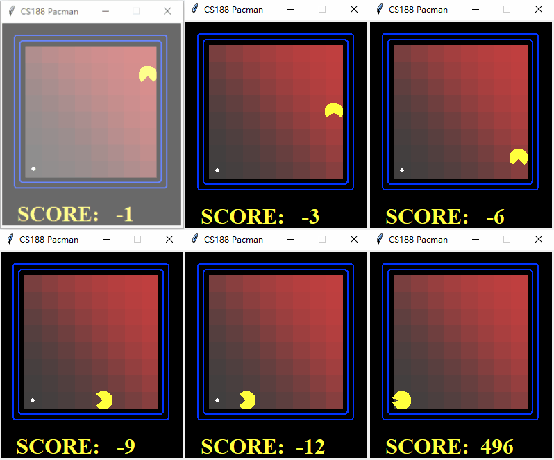
One can see that the agent using BFS reaches the endpoint via the shortest path because BFS is both complete and optimal.
Iterative Deepening Search
IDS works by repeatedly performing a DFS with a limited depth to find the optimal solution. It combines the advantages of DFS (space complexity) and BFS (completeness and optimality), but it performs poorly in terms of time complexity (refer to the Search nodes expanded in the output results).
def IterativeDeepeningSearch(problem):
    import sys
    from util import Stack

    def depthLimitSearch(problem, depth):
        visited = []
        open_list = Stack()
        open_list.push((problem.getStartState(), [], visited))
        while not open_list.isEmpty():
            current_node, path, visited = open_list.pop()
            if problem.isGoalState(current_node):
                return path
            if len(path) == depth or depth == 0:
                continue
            if current_node in visited:
                continue
            actions = problem.getSuccessors(current_node)
            for next_node, action, cost in actions:
                if next_node not in visited:
                    open_list.push((next_node, path + [action], visited+[current_node]))

    for depth in range(sys.maxsize**10):
        path = depthLimitSearch(problem, depth)
        if path:
            return path

ids = IterativeDeepeningSearch
This algorithm performs well on maps with a small searchable area:
$ python pacman.py -l smallMaze -z 0.8 -p SearchAgent -a fn=ids
[SearchAgent] using function ids
[SearchAgent] using problem type PositionSearchProblem
Path found with total cost of 19 in 0.008976 seconds
Search nodes expanded: 923
Pacman emerges victorious! Score: 491
Average Score: 491.0
Scores:        491.0
Win Rate:      1/1 (1.00)
Record:        Win
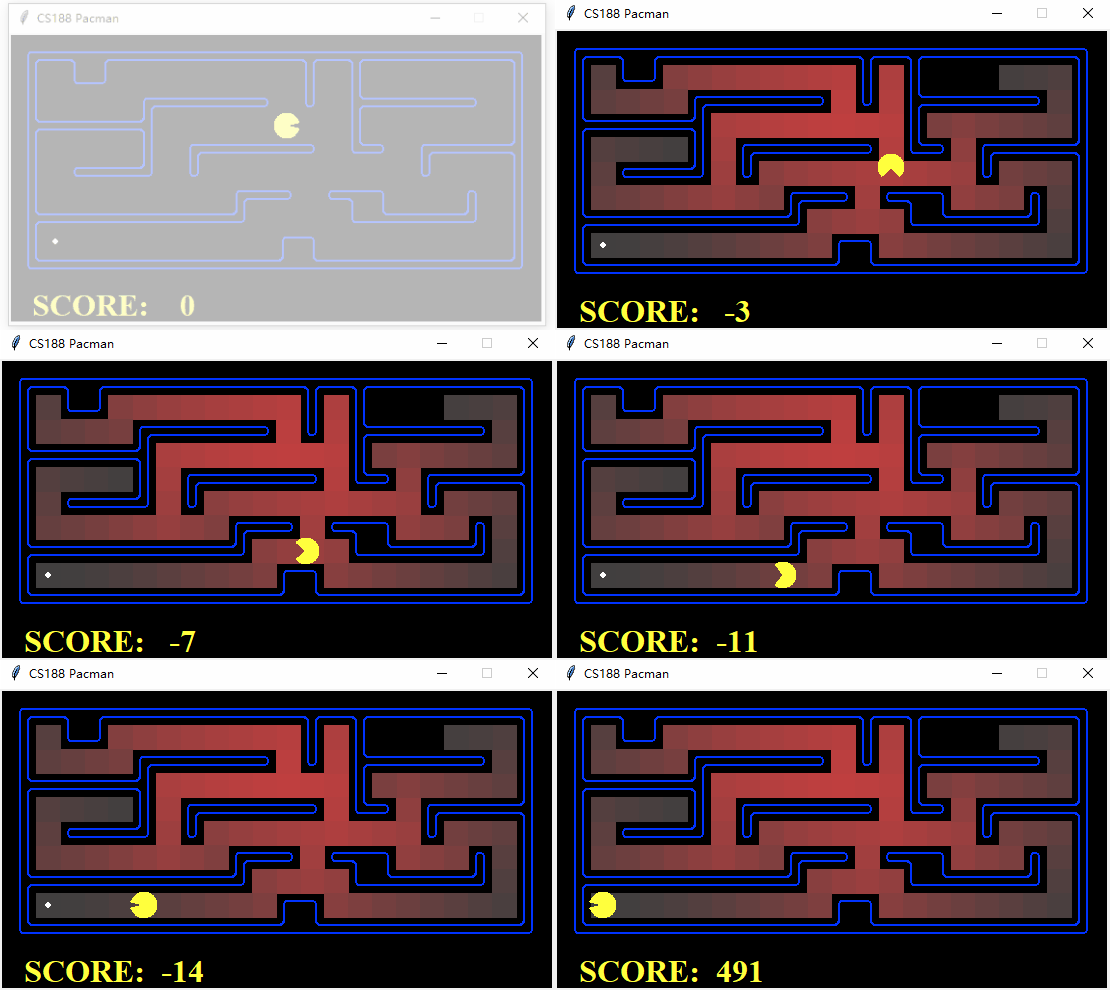
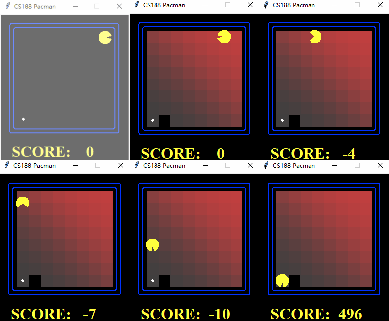
For maps with large searchable areas, the search process will take a very long time.
$ python pacman.py -l smallEmpty -z 0.8 -p SearchAgent -a fn=ids
[SearchAgent] using function ids
[SearchAgent] using problem type PositionSearchProblem
Path found with total cost of 14 in 0.710854 seconds
Search nodes expanded: 94552
Pacman emerges victorious! Score: 496
Average Score: 496.0
Scores:        496.0
Win Rate:      1/1 (1.00)
Record:        Win
Uniform Cost Search
UCS and Dijkstra are similar, maintaining a priority queue that stores the cost from the starting node to each node. It sequentially expands the node with the minimum path cost until the endpoint is reached. Unlike Dijkstra, which generally does not have a fixed endpoint.
def UniformCostSearch(problem):
    from util import PriorityQueue
    frontier = PriorityQueue()
    visited = []
    frontier.push((problem.getStartState(), [], 0), 0)
    while not frontier.isEmpty():
        current_node, path, current_cost = frontier.pop()
        if problem.isGoalState(current_node):
            return path
        if current_node in visited:
            continue
        visited.append(current_node)
        for next_node, action, cost in problem.getSuccessors(current_node):
            if next_node not in visited:
                frontier.push((next_node, path + [action], current_cost + cost), current_cost + cost)
ucs = UniformCostSearch
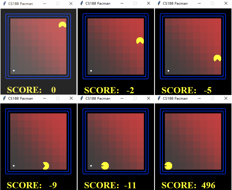
$ python pacman.py -l smallEmpty -z 0.8 -p SearchAgent -a fn=ucs
[SearchAgent] using function ucs
[SearchAgent] using problem type PositionSearchProblem
Path found with total cost of 14 in 0.002992 seconds
Search nodes expanded: 63
Pacman emerges victorious! Score: 496
Average Score: 496.0
Scores:        496.0
Win Rate:      1/1 (1.00)
Record:        Win
2 Heuristic Search
Traditional blind search algorithms are rarely used in practical applications due to factors such as completeness, optimality, time, and space complexity. In path planning, optimization algorithms, and artificial intelligence, Heuristic Search (Informed Search) can better balance accuracy and computational speed.
Heuristic Search differs from blind search in two aspects: Firstly, it relies on a heuristic function, which is a type of function used to estimate the distance from the current node to the target node; Secondly, it requires the use of input data and treats it as a parameter for the heuristic function to measure the distance relationship between the current position and the target position.
Heuristic Search directs the search process to move towards directions closer to the target position to improve efficiency.
Heuristic Function
The heuristic function ( h(n) ) provides an estimated value (not the actual value) of the distance from a specific node to the target node. Many path-finding problems are NP-complete, meaning their algorithm time complexity is exponential in the worst case. Finding a good heuristic function can lead to more efficient and better solutions. The quality of the heuristic function directly determines the efficiency of the informed search.
The simplest heuristic functions include:
- null heuristic: The estimated value is always 0, effectively degenerating into UCS (only calculating the distance from the current node to the start node);
- Manhattan distance: The sum of the distances in the north-south direction and the east-west direction, i.e., ( |a - x| + |b - y| );
- Euclidean distance: The straight-line distance in the Euclidean space, i.e., ( \sqrt{(a - x)^2 + (b - y)^2} );
A*
A* is a widely applied heuristic search algorithm, similar to Dijkstra and UCS in its main idea of utilizing a priority queue to repeatedly extract the top node and determine whether it is the target node. The difference lies in that it computes the sum of the actual distance from the start to the current node, g(x), and the heuristic estimate of the distance from the current node to the target node, h(x), to form the function f(x) = g(x) + h(x).
def AStarSearch(problem, heuristic=nullHeuristic):
    from util import PriorityQueueWithFunction
    def AStarHeuristic(item):
        state, _, cost = item
        h = heuristic(state, problem=problem)
        g = cost
        return g + h

    frontier = PriorityQueueWithFunction(AStarHeuristic)
    visited = []

    frontier.push((problem.getStartState(),[], 0))
    while not frontier.isEmpty():
        currentNode, path, currentCost = frontier.pop()
        if problem.isGoalState(currentNode):
            return path
        if currentNode not in visited:
            visited.append(currentNode)
            for nextNode, action, cost in problem.getSuccessors(currentNode):
                if nextNode not in visited:
                    frontier.push((nextNode, path + [action], currentCost + cost))

astar = AStarSearch
For multi-node search problems, we need to consider the impact of all target nodes on the current node. We can use a greedy approach, where Pac-Man prioritizes moving towards the closest beans, i.e., making the heuristic value of target nodes closer to the current node smaller. This ensures that beans closer to Pac-Man are more likely to have a smaller f(x) value. In the heuristic function, state is a tuple containing the current position position and target point information grid. We can use grid.asList() to convert all target points into an array.
def FoodHeuristic(state, problem):
    position, food_grid = state
    food_gridList = food_grid if isinstance(food_grid, list) else food_grid.asList()
    from util import manhattanDistance
    minx, miny = position
    maxx, maxy = position
    for food in food_gridList:
        foodx, foody = food
        minx = min(foodx,minx)
        maxx = max(foodx,maxx)
        miny = min(foody,miny)
        maxy = max(foody,maxy)
    return abs(minx-maxx) + abs(miny-maxy)
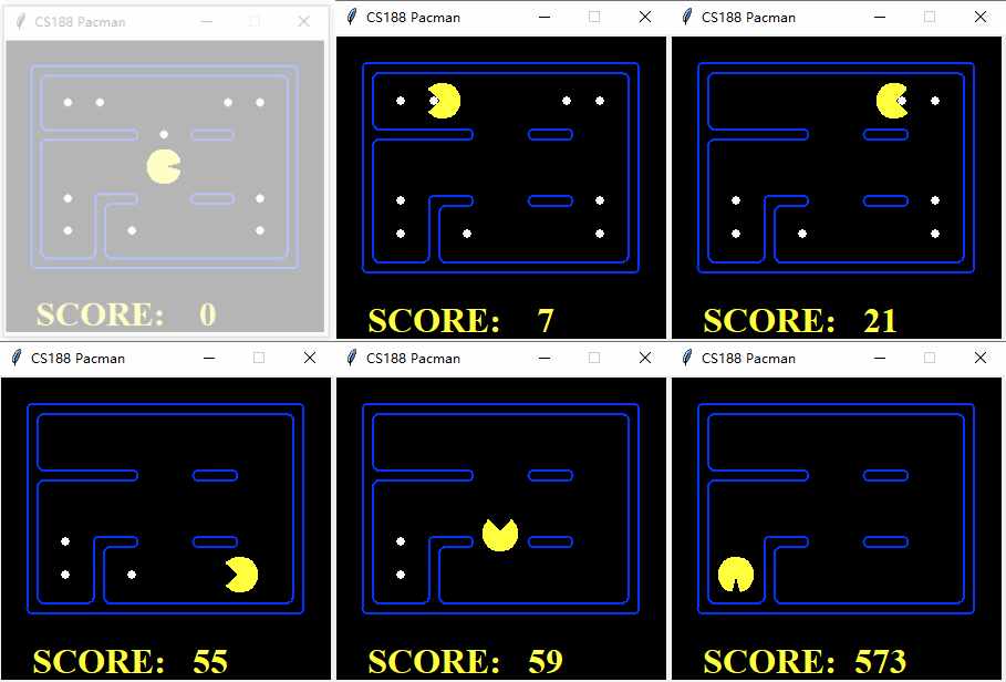
$ python pacman.py -l tinySearch -p SearchAgent -a fn=astar,prob=FoodSearchProblem,heuristic=FoodHeuristic
[SearchAgent] using function astar and heuristic foodHeuristic
[SearchAgent] using problem type FoodSearchProblem
Path found with total cost of 27 in 0.294214 seconds
Search nodes expanded: 1544
Pacman emerges victorious! Score: 573
Average Score: 573.0
Scores:        573.0
Win Rate:      1/1 (1.00)
Record:        Win
Replace the map with a different one to see the effect:
$ python pacman.py -l mediumDottedMaze -p SearchAgent -a fn=astar,prob=FoodSearchProblem,heuristic=FoodHeuristic
[SearchAgent] using function astar and heuristic foodHeuristic
[SearchAgent] using problem type FoodSearchProblem
Path found with total cost of 74 in 0.091756 seconds
Search nodes expanded: 389
Pacman emerges victorious! Score: 646
Average Score: 646.0
Scores:        646.0
Win Rate:      1/1 (1.00)
Record:        Win

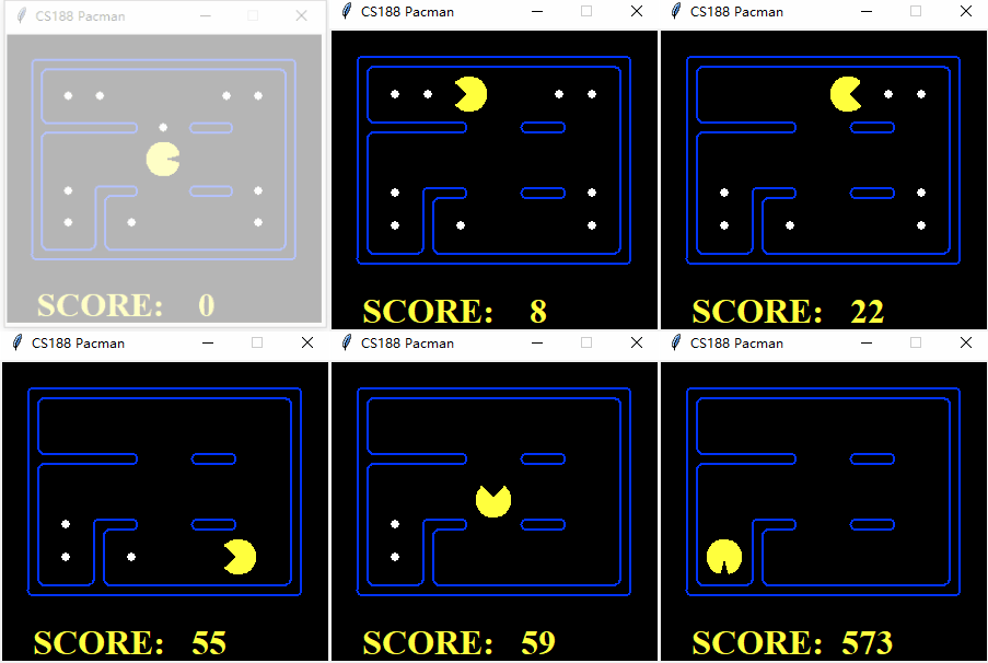
In fact, using nullHeuristic (degenerate UCS) would make the search take much longer.
$ python pacman.py -l tinySearch -p SearchAgent -a fn=ucs,prob=FoodSearchProblem
[SearchAgent] using function ucs
[SearchAgent] using problem type FoodSearchProblem
Path found with total cost of 27 in 2.880744 seconds
Search nodes expanded: 5057
Pacman emerges victorious! Score: 573
Average Score: 573.0
Scores:        573.0
Win Rate:      1/1 (1.00)
Record:        Win
3 Reinforcement Learning
Reinforcement Learning
Reinforcement learning is a process where an entity, referred to as agent, learns a strategy through interaction and feedback with an environment. During this process, the agent interacts with the environment and takes a series of actions to achieve a certain reward, thereby updating the weights corresponding to these actions.
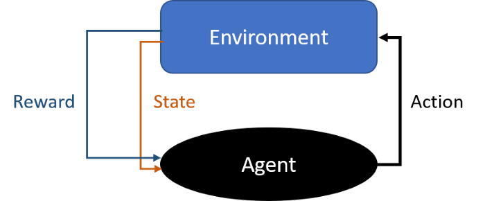
The goal of reinforcement learning is to learn a policy Policy such that the agent maximizes the long-term reward. Therefore, in most problems, the reward is typically negative (decreasing over time) until the final goal is achieved, at which point a large positive feedback is received. Such learning tasks are often referred to as episodic tasks (such as single-node search problems in games like Pac-Man); in another category of problems, multiple goals need to be achieved to reach the final state, with the reward being distributed discretely over a continuous space. These tasks are called continuing tasks (such as multi-node search problems in games like Pac-Man). For continuing tasks, we can define the reward as:
 Where $\gamma$ is the discount factor, which makes us more inclined towards immediate rewards. There are many reasons for introducing the discount coefficient, such as avoiding infinite loops, reducing uncertainty of distant rewards, maximizing immediate rewards, generating new rewards through immediate rewards, making them more valuable, and so on.
While the result of reinforcement learning is Gt, the value obtained through argmax gives the action we should take in each state. We can denote this strategy as π(a|s), which represents the probability of taking action a in state s.
Markov Decision Processes
Markov Decision Process (MDP) refers to the selection of actions by an agent in each state that depends solely on the current state and not on any previous actions. Almost all reinforcement learning problems can be addressed using MDPs. A standard Markov Decision Process consists of a quadruple:
- S: State, the set of state spaces, S0 represents the initial state;
- A: Action, the set of action spaces, containing actions that can be performed from each state;
- r(s’ | s, a): Reward, the reward obtained when transitioning from state s to state s’ under action a;
- P(s’ | s, a): Probability, the probability of transitioning from state s to state s’ under action a;
Common methods for solving MDP problems include Value iteration, Policy iteration, Q-Learning, and Deep Q-Learning Network, etc.
Value Iteration
Value Iteration is a model-based algorithm that resolves MDP problems via Value Iteration, provided that we have all information about the model, which comprises the entirety of the MDP quadruplet.
Assuming there is a $3 \times 4$ map called GridWorld as shown in the diagram below, with the bottom-left corner at $(0, 0)$, where $(1, 1)$ is an impassable wall, $(2, 3)$ is a goal with a reward of $+1$, and $(1, 3)$ is a goal with a reward of $-1$. We define the value of each state $V(state)$, which represents the maximum value that can be obtained from state $(x, y)$. Initially, the value of each state is set to $0$:
GridWorld: (0, 0) (0, 1) (0, 2) (1, 0) (1, 1) (1, 2) (2, 0) (2, 1) (2, 2)
// Value initialization V((0, 0)) = 0 V((0, 1)) = 0 V((0, 2)) = 0 V((1, 0)) = 0 V((1, 1)) = 0 V((1, 2)) = 0 V((2, 0)) = 0 V((2, 1)) = 0 V((2, 2)) = 0

During the iteration process, the Bellman equation is used to update the value for all positions. It describes the condition that the optimal strategy must satisfy, where the part r(s, a, s') represents the reward obtained after taking the action a, and the part afterward. We need to compute the value of each state, V(s), at each iteration until the difference between two consecutive iterations is less than a given threshold. This value, V(s), is also referred to as the q-value.
 After three iterations, we obtain:
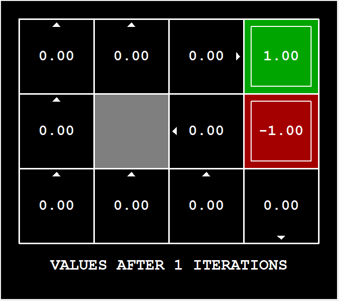
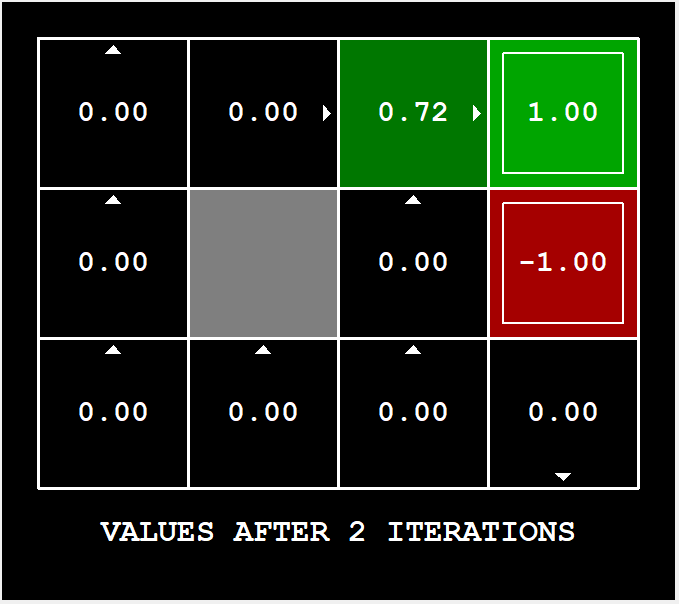
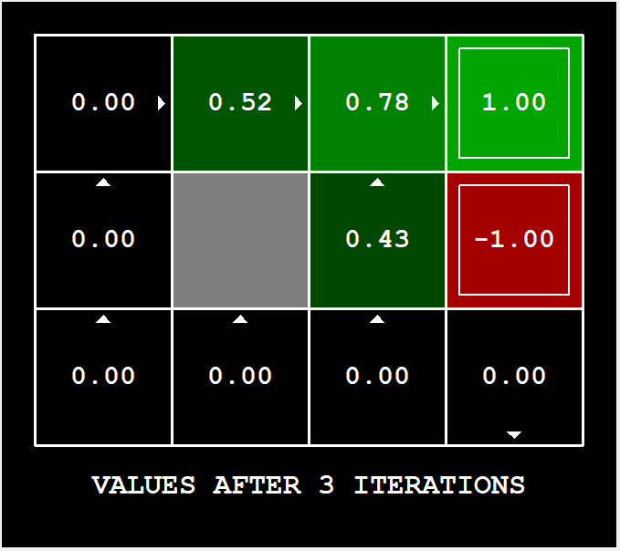
Convergence speed is exponential, and eventually, the optimal V(s) will be obtained through continuous iterations; or, to put it another way, the optimal solution for V(s) will be achieved as the number of iterations approaches infinity; after 100 iterations, we will have:

Take the argmax to obtain the optimal strategy (as indicated by the small arrow in the figure above); one can also see the Probability corresponding to each action taken.
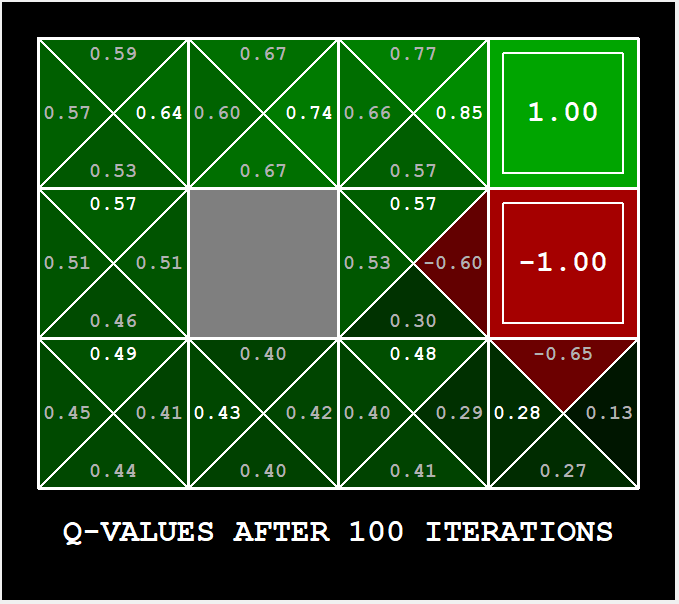
The process of Value Iteration corresponds to the functions runValueIteration and computeQValueFromValues. After the iteration ends, the strategy is computed using the function computeActionFromValues.
# valueIterationAgents.py

class ValueIterationAgent(ValueEstimationAgent):
    """
        A ValueIterationAgent takes a Markov decision process
        (see mdp.py) on initialization and runs value iteration
        for a given number of iterations using the supplied
        discount factor.
    """
    def __init__(self, mdp, discount = 0.9, iterations = 100):
        """
          Some useful mdp methods you will use:
              mdp.getStates()
              mdp.getPossibleActions(state)
              mdp.getTransitionStatesAndProbs(state, action)
              mdp.getReward(state, action, nextState)
              mdp.isTerminal(state)
        """
        self.mdp = mdp
        self.discount = discount
        self.iterations = iterations
        self.values = util.Counter() # A Counter is a dict with default 0
        self.runValueIteration()

    def runValueIteration(self):
        for _ in np.arange(0, self.iterations):
            next_values = util.Counter()

            for state in self.mdp.getStates():
                if self.mdp.isTerminal(state):
                    continue

                q_values = util.Counter()

                for action in self.mdp.getPossibleActions(state):
                    q_values[action] = self.computeQValueFromValues(state, action)

                key_max_value = q_values.argMax()
                next_values[state] = q_values[key_max_value]

            self.values = next_values

    def getValue(self, state):
        return self.values[state]


    def computeQValueFromValues(self, state, action):
        """
          Compute the Q-value of action in state from the
          value function stored in self.values.
        """
        next_states_probs = self.mdp.getTransitionStatesAndProbs(state, action)
        q_value = 0

        for (next_state, next_state_prob) in next_states_probs:
            q_value += next_state_prob * (self.mdp.getReward(state, action, next_state) + self.discount * self.values[next_state])

        return q_value

    def computeActionFromValues(self, state):
        """
          The policy is the best action in the given state
          according to the values currently stored in self.values.

          You may break ties any way you see fit.  Note that if
          there are no legal actions, which is the case at the
          terminal state, you should return None.
        """
        if self.mdp.isTerminal(state):
            return None

        actions = self.mdp.getPossibleActions(state)
        values = util.Counter()

        for action in actions:
            values[action] = self.computeQValueFromValues(state, action)

        policy = values.argMax()
        return policy


    def getPolicy(self, state):
        return self.computeActionFromValues(state)

    def getAction(self, state):
        "Returns the policy at the state (no exploration)."
        return self.computeActionFromValues(state)

    def getQValue(self, state, action):
        return self.computeQValueFromValues(state, action)
Q-Learning
Q-Learning has some similarities with Value Iteration, but it is a model-free algorithm. In Q-Learning, our agent does not need to know the current environment’s state, action, and other MDP quadruplets beforehand.
When using Value Iteration, we need to update all the states and actions for every episode. However, in actual problems, the number of states can be very large, making it impractical to traverse all states. In such cases, we can leverage Q-Learning. Without prior knowledge of the environment, we can interact with the environment and explore it repeatedly. We can compute Q-Values based on a limited set of environment samples and maintain a Q-Table.
| S | r(s’ | s, action 1) | r(s’ | s, action 2) | … |
|---|---|---|---|
| S1 (0, 0) | 3 | -1 | |
| S2 (0, 1) | -2 | 4 | |
| … |
At the beginning, the agent knows nothing about the environment, so the Q-Table should be initialized as a zero matrix. When in a state s (such as S1), the optimal value in the Q-Table and a certain strategy (e.g., a Multi-armed bandit problem, using ε-greedy or UCB methods) are used to select action a (say action 1, resulting in reward r = 3). Exploration is then conducted based on this reward, and the immediate reward r is used to update the reward. Here, r is the immediate reward (3), but future maximum reward r’ (4) might be obtained in the next state s’ (such as S2).
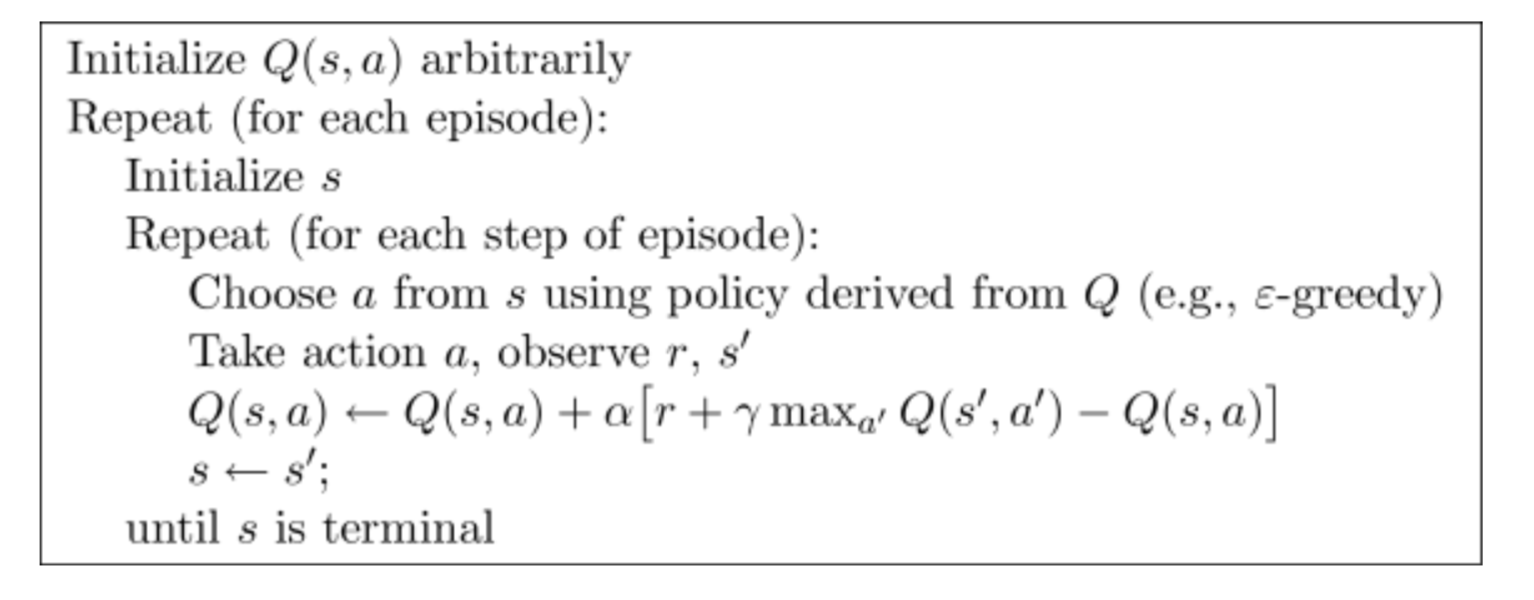
The true reward Q(St, At) is composed of two parts in the formula, the front part r is the immediate reward obtained by action a (i.e., r = 3), and the back part γ * max(a’)Q(s’, a’) is the maximum expected reward for future actions (i.e., r’ = 4), and the back part is often uncertain, hence it needs to be multiplied by the decay rate γ:

After calculating the expected reward that the current behavior can obtain, it is subtracted from the estimated reward Q(s,a) in the table for the current environment, and then multiplied by the learning rate to update the value in the Q-Table.
The agent continuously explores and experiences state transitions with the environment until it reaches the target; we refer to each exploration of the agent (starting from any initial state and experiencing several actions until reaching the target state) as an episode; after training for a specified number of episodes, the strategy obtained by taking the argmax is the current optimal solution.
Now, we use epsilon-greedy as the exploration strategy and train for 10 episodes.
$ python gridworld.py -a q -k 10 --noise 0.0 -e 0.9

After obtaining the result, taking the argmax over all actions (a) for every state (s) yields the optimal solution under the current epsilon value and episode value:
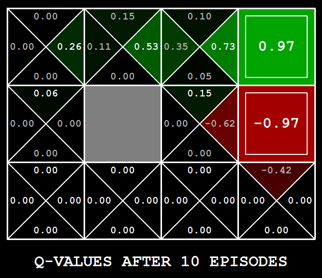
Q-Learning implementation roughly looks like this:
class QLearningAgent(ReinforcementAgent):
    def __init__(self, **args):
        ReinforcementAgent.__init__(self, **args)
        self.q_values = defaultdict(lambda: 0.0)

    def getQValue(self, state, action):
        """
          Returns Q(state,action)
          Should return 0.0 if we have never seen a state
          or the Q node value otherwise
        """
        return self.q_values[(state, action)]

    def computeValueFromQValues(self, state):
        """
          Returns max_action Q(state,action)
          where the max is over legal actions.  Note that if
          there are no legal actions, which is the case at the
          terminal state, you should return a value of 0.0.
        """
        next_actions = self.getLegalActions(state)

        if not next_actions:
            return 0.0
        else:
            q_value_actions = [(self.getQValue(state, action), action) for action in next_actions]
            # return the max in q_value_actions which is q_value
            return sorted(q_value_actions, key=lambda x: x[0])[-1][0]

    def computeActionFromQValues(self, state):
        """
          Compute the best action to take in a state.  Note that if there
          are no legal actions, which is the case at the terminal state,
          you should return None.
        """
        next_actions = self.getLegalActions(state)

        if not next_actions:
            return None
        else:
            actions = []
            max_q_value = self.getQValue(state, next_actions[0])

            # find actions with max q value
            for action in next_actions:
                action_q_value = self.getQValue(state, action)
                if max_q_value < action_q_value:
                    max_q_value = action_q_value
                    actions = [action]
                elif max_q_value == action_q_value:
                    actions.append(action)

            # break ties randomly for better behavior. The random.choice() function will help.
            return random.choice(actions)

    def getAction(self, state):
        """
          Compute the action to take in the current state.  With
          probability self.epsilon, we should take a random action and
          take the best policy action otherwise.  Note that if there are
          no legal actions, which is the case at the terminal state, you
          should choose None as the action.
        """
        # Pick Action
        legalActions = self.getLegalActions(state)
        action = None
        if legalActions:
            if util.flipCoin(self.epsilon):
                return random.choice(legalActions)
            else:
                action = self.getPolicy(state)

        return action

    def update(self, state, action, nextState, reward):
        """
          The parent class calls this to observe a
          state = action => nextState and reward transition.
          You should do your Q-Value update here

          NOTE: You should never call this function,
          it will be called on your behalf
        """
        state_action_q_value = self.getQValue(state, action)
        self.q_values[(state, action)] = state_action_q_value + self.alpha * (reward + self.discount * self.getValue(nextState) - state_action_q_value)

    def getPolicy(self, state):
        return self.computeActionFromQValues(sta、te)

    def getValue(self, state):
        return self.computeValueFromQValues(state)
DQN
Q-Learning relies on a Q-Table, and its limitation is that when the Q-Table has a large number of states or high dimensions, it may not be able to store all states in memory. In this case, we can use a neural network to approximate the entire Q-Table, which is known as Deep Q-Learning Network. DQN is primarily used to solve problems where the State is nearly infinite but the Action is limited. It takes the current State as input and outputs the Q-Value for each Action.
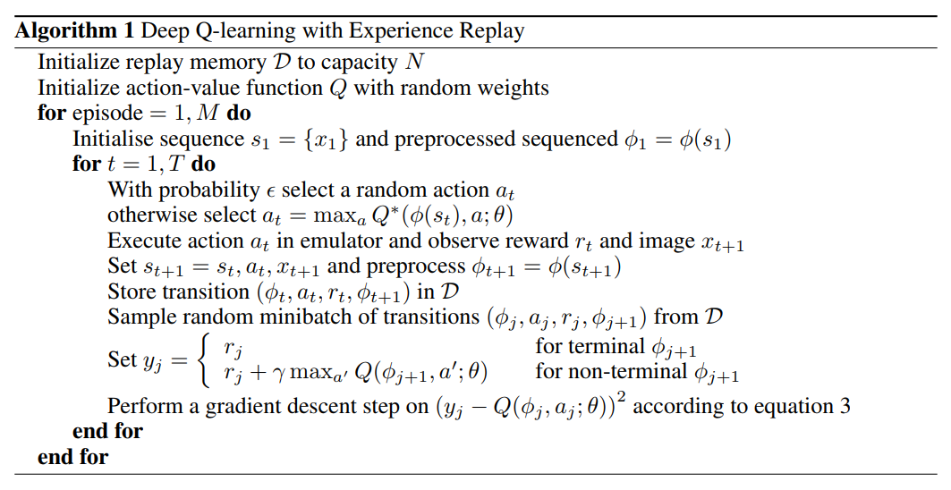
Heuristic Search and Reinforcement Learning Comparison